6. Advanced features of the mobest package
mobest::locate() uses spatiotemporal interpolation to calculate spatial similarity probability maps between a set of search samples and an interpolated ancestry field at specific time slices. This basic and arguably most important use case of the mobest package is documented in A basic similarity search workflow. locate() hides a lot of the complexity of mobest, though, and some of that is unveiled in the following sections.
6.1. Gaussian process regression on top of a linear model
An important detail of mobest is that it typically performs the spatiotemporal interpolation for an individual dependent variable in a two-step process. It starts with a simple linear model that predicts the dependent variable based on the three independent space and time variables, thus detrending the entire dataset. The more advanced, complex and computationally expensive Gaussian process regression model is then only applied to the residuals of the linear models.
Here is how this is implemented in mobest:::interpolate():
if (on_residuals) {
    combined <- independent %>% dplyr::mutate(d = dependent)
    model <- stats::lm(d ~ x + y + z, data = combined)
    dependent <- model[["residuals"]]
  }
The detrending step can be turned off for individual variables in mobest::create_kernel(), by setting on_residuals = FALSE (see Kernel parameter settings).
6.2. Spatiotemporal interpolation permutations in a model grid
Spatiotemporal interpolation is the first main operation mobest undertakes. The actual interpolation is performed in an internal function mobest:::interpolate(), which has a minimal interface and does not have to be called directly by the user. This is not least, because the main workflow in mobest::locate() (see A basic similarity search workflow) generally requires multiple interpolation runs. mobest therefore offers a slightly more complex, two step interpolation workflow, which consists of the creation of a list of models and then subsequently running each element in this list to construct different ancestry fields.
mobest::create_model_grid() creates an object of class mobest_modelgrid which holds all permutations of the field-defining input objects. Each row equals one complete model definition with all parameters and input data fully defined. Here is how this function is called with the necessary input data constructors:
library(magrittr)
model_grid <- mobest::create_model_grid(
  independent     = mobest::create_spatpos_multi(...),
  dependent       = mobest::create_obs_multi(...),
  kernel          = mobest::create_kernset_multi(...),
  prediction_grid = mobest::create_spatpos_multi(...)
)
Warning
Unlike for locate() we here require the *_multi constructors to express iterations of all settings (for more about this see Similarity search with permutations below).
This model grid is only a specification of the models we want to run, so the interpolated fields we want to create. It features the following columns, some of which are list columns including the concrete data to inform the desired interpolation.
Column |
Description |
|---|---|
independent_table_id |
Identifier of the spatiotemporal position permutation |
dependent_setting_id |
Identifier of the dependent variable space position permutation |
dependent_var_id |
Identifier of the dependent variable |
kernel_setting_id |
Identifier of the kernel setting permutation |
pred_grid_id |
Identifier of the spatiotemporal prediction grid |
independent_table |
List column: |
dependent_var |
List column: |
kernel_setting |
List column: |
pred_grid |
List column: |
Another function, mobest::run_model_grid(), then takes this model_grid object and runs each interpolation.
interpol_grid <- mobest::run_model_grid(model_grid, quiet = T)
It returns an unnested table of type mobest_interpolgrid, where each row documents the result of the interpolation for one prediction grid point and each parameter setting. It includes the following columns/variables: independent_table_id, dependent_setting_id, dependent_var_id, kernel_setting_id, pred_grid_id, dsx, dsy, dt, g, id, x, y, z, mean, sd.
These are identical to what we already know from the output of mobest::locate() (see The mobest_locateoverview table) or mobest::crossvalidate() (see A basic crossvalidation setup). This is simply, because these functions internally call create_model_grid() and run_model_grid() and build their own output on top of the mobest_interpolgrid structure.
6.3. Similarity search with permutations
As already pointed out in The mobest_locateoverview table, mobest::locate() is a special, simplified interface for mobest::locate_multi(). This more general function adds another level of complexity, by allowing multiple input values for independent, dependent, kernel, search_independent and search_dependent through a set of data types and constructor functions with the suffix *_multi (see Permutation data types). The result will consider all permutations of these input settings (independent and search_independent as well as dependent and search_dependent have to be congruent, though).
library(magrittr)
search_result <- mobest::locate_multi(
  independent        = mobest::create_spatpos_multi(...),
  dependent          = mobest::create_obs_multi(...),
  kernel             = mobest::create_kernset_multi(...),
  prediction_grid    = mobest::create_spatpos(...),
  search_independent = mobest::create_spatpos_multi(...),
  search_dependent   = mobest::create_obs_multi(...),
  search_space_grid  = mobest::create_spatpos(...),
  search_time        = 0,
  search_time_mode   = "relative"
)

search_product <- mobest::multiply_dependent_probabilities(search_result)
The result of locate_multi() is also an object of type mobest_locateoverview, just as for locate(). But locate_multi() actually makes use of its columns independent_table_id, dependent_setting_id, dependent_var_id and kernel_setting_id.
So locate_multi() produces potentially many probability grids for each sample. Even after the per-dependent variable iterations are merged with mobest::multiply_dependent_probabilities(), that could still leave many parameter permutations. mobest::fold_probabilities_per_group() is a convenient function to combine these into a single, merged probability grid of class mobest_locatefold. The folding operation for the probability densities can be set in the argument folding_operation, where the default is a simple sum. Again, in the default setting, the output probabilities are normalized per permutation.
mobest::fold_probabilities_per_group(search_product)
fold_probabilities_per_group also allows to maintain all or some permutation groups, in case a full summary is not desired, for example:
mobest::fold_probabilities_per_group(search_product, dependent_setting_id, kernel_setting_id)
6.3.1. Temporal resampling as a permutation application
The introduction of mobest::locate_multi() above has been abstract and devoid of any hint to the great power that comes with its permutation machinery. Here we want to show one application that is very relevant for archaeogenetic and macro-archaeological applications of mobest: Temporal resampling.
Samples extracted from archaeological contexts usually have no precise age information that would allow them to be pin-pointed to exactly one year. Instead they can either be linked to a certain age range through relative chronology based on stratigraphy or typology, or they are dated with biological, physical or chemical methods of dating like, most prominently, radiocarbon dating. No matter how ingenious the method of dating might be, even including sophisticated chronological modelling based on various lines of evidence, the outcome for the individual sample will almost always be a probability distribution over a set of potential years. And this set can be surprisingly large - up to several hundred years - with highly asymmetric probability distributions.
As a consequence, spatiotemporal interpolation only based on the median age, as demonstrated in A basic similarity search workflow, is of questionable accuracy. The following section introduces a modified version of this simple workflow, now featuring temporal resampling based on archaeological age ranges and radiocarbon dates.
We start again by downloading and sub-setting data from [Schmid and Schiffels, 2023]. Here we already perform some additional steps in advance to reduce the complexity a bit. This includes the transformation of the spatial coordinates and the parsing and restructuring of the uncalibrated radiocarbon dates.
Code to prepare the input data table.
# download .zip archives with tables from https://doi.org/10.17605/OSF.IO/6UWM5
utils::download.file(
  url = "https://osf.io/download/kej4s/",
  destfile = "docs/data/pnas_tables.zip"
)
# extract the relevant tables
utils::unzip(
  "docs/data/pnas_tables.zip",
  files = c("Dataset_S1.csv", "Dataset_S2.csv"),
  exdir = "docs/data/"
)
# read data files
samples_context_raw <- readr::read_csv("docs/data/Dataset_S1.csv")
samples_genetic_space_raw <- readr::read_csv("docs/data/Dataset_S2.csv")
# join them by sample name
samples_raw <- dplyr::left_join(
  samples_context_raw,
  samples_genetic_space_raw,
  by = "Sample_ID"
)
# create a useful subsets of this table
samples_selected <- samples_raw %>%
  dplyr::select(
    Sample_ID,
    Latitude, Longitude,
    Date_BC_AD_Start, Date_BC_AD_Median, Date_BC_AD_Stop, Date_C14,
    MDS_C1 = C1_mds_u, MDS_C2 = C2_mds_u
  )
# transform the spatial coordinates to EPSG:3035
samples_projected <- samples_selected %>%
  sf::st_as_sf(coords = c("Longitude", "Latitude"), crs = 4326) %>%
  sf::st_transform(crs = 3035) %>%
  dplyr::mutate(
    x = sf::st_coordinates(.)[,1],
    y = sf::st_coordinates(.)[,2],
    .after = "Sample_ID"
  ) %>%
  sf::st_drop_geometry()
# restructure radiocarbon information
samples_advanced <- samples_projected %>%
  tibble::add_column(
    .,
    purrr::map_dfr(
      .$Date_C14,
      function(y) {
        tibble::tibble(
          C14_ages = paste(stringr::str_match_all(y, ":(.*?)±")[[1]][,2], collapse = ";"),
          C14_sds = paste(stringr::str_match_all(y, "±(.*?)\\)")[[1]][,2], collapse = ";")
        )
      }
    ),
    .after = "Date_C14"
  )
readr::write_csv(samples_advanced, file = "docs/data/samples_advanced.csv")
You do not have to run this and can instead download the example table samples_advanced.csv here. Additional to the simple Date_BC_AD_Median column this table has a different set of variables to express age:
Variable |
Type |
Description |
|---|---|---|
Date_BC_AD_Start |
int |
The start of the age range for this sample in years BC/AD |
Date_BC_AD_Stop |
int |
The end of the age range for this sample in years BC/AD |
Date_C14 |
chr |
A list of radiocarbon dates for each sample |
C14_ages |
chr |
A string list with only the BP ages of the C14 dates |
C14_sds |
chr |
A string list with only the standard deviations of the C14 dates |
With samples_advanced.csv we can write code to draw age samples and then use them for the similarity search. The script and the data can be downloaded here:
The snapshot includes some R objects created in A basic similarity search workflow.
6.3.1.1. Drawing ages for each sample
As expected we start this analysis by loading the relevant dependencies and data.
library(magrittr)
library(ggplot2)

samples_advanced <- readr::read_csv("docs/data/samples_advanced.csv")
The first step to draw age samples is then to determine per-year probability densities for each sample. For the ones without radiocarbon dates this density follows a simple, uniform distribution. We assign each year a fraction, depending on the total number of years between Date_BC_AD_Start and Date_BC_AD_Stop. We can encode this algorithm in a simple helper function contextual_date_uniform(), which returns a tibble with the years in a column age and the respective densities in a column sum_dens.
contextual_date_uniform <- function(startbcad, stopbcad) {
  tibble::tibble(
    age = startbcad:stopbcad,
    sum_dens = 1/(length(startbcad:stopbcad))
  )
}
For the samples with radiocarbon ages this is more involved, because we have to calibrate the radiocarbon ages and determine the normalized sum of their post-calibration probability density distributions.
For the calibration we use the Bchron R package [Haslett and Parnell, 2008], which implements a simple, fast calibration algorithm. We then sum the per-year densities in case there are multiple uncalibrated dates for a given sample, normalize them and fill age range gaps in the Bchron::BchronCalibrate() output (some years fall below its density threshold) with 0 to get a continuos sequence of years and densities. The output of radiocarbon_date_sumcal() has the same structure as produced by contextual_date_uniform(): a tibble with the years in a column age and densities in a column sum_dens.
radiocarbon_date_sumcal <- function(ages, sds, cal_curve) {
  bol <- 1950 # c14 reference zero
  raw_calibration_output <- Bchron::BchronCalibrate(
    ages      = ages,
    ageSds    = sds,
    calCurves = rep(cal_curve, length(ages))
  )
  density_tables <- purrr::map(
    raw_calibration_output,
    function(y) {
      tibble::tibble(
        age = as.integer(-y$ageGrid + bol),
        densities = y$densities
      )
    }
  )
  sum_density_table <- dplyr::bind_rows(density_tables) %>%
    dplyr::group_by(age) %>%
    dplyr::summarise(
      sum_dens = sum(densities)/length(density_tables),
      .groups = "drop"
    ) %>%
    dplyr::right_join(
      ., data.frame(age = min(.$age):max(.$age)), by = "age"
    ) %>%
    dplyr::mutate(sum_dens = tidyr::replace_na(sum_dens, 0)) %>%
    dplyr::arrange(age)
  return(sum_density_table)
}
With these helper functions we can modify samples_advanced to include a new list-column Date_BC_AD_Prob, which features the density tibbles for each sample.
Warning
Running this code can take several minutes, because it involves thousands of radiocarbon calibration operations.
samples_with_age_densities <- samples_advanced %>%
  dplyr::mutate(
    Date_BC_AD_Prob = purrr::pmap(
      list(Date_BC_AD_Start, Date_BC_AD_Stop, C14_ages, C14_sds),
      function(context_start, context_stop, c14bps, c14sds) {
        if (!is.na(c14bps)) {
          radiocarbon_date_sumcal(
            ages = as.numeric(strsplit(c14bps, ";")[[1]]),
            sds = as.numeric(strsplit(c14sds, ";")[[1]]),
            cal_curve = "intcal20"
          )
        } else {
          contextual_date_uniform(
            startbcad = context_start,
            stopbcad = context_stop
          )
        }
      }
    )
  )
Note that we set the calibration curve for all samples to cal_curve = "intcal20". This is a sensible default for Western Eurasia, but not necessarily for other parts of the world.
Warning
The calibration-based age probabilities we generate in this script are an improvement over using just median ages. But they still equate to a massive simplification of the per-sample age information. Each individual sample could potentially be informed by a dedicated chronological model to make the derived pear-year probabilities much more accurate and precise. But such models are typically only available for individual sites and not for large meta-datasets like the ones required for spatiotemporal interpolation on a continental scale.
In a last step we can define the number of age resampling runs we want to apply and draw this number of random samples from the age distributions for each sample. For the example here we chose two, but for a real world application a larger number (>50) is recommended.
age_resampling_runs <- 2 # only two in this minimal example

set.seed(123)

samples_with_age_samples <- samples_with_age_densities %>%
  dplyr::mutate(
    Date_BC_AD_Samples = purrr::map(
      Date_BC_AD_Prob, function(x) {
        sample(
          x    = x$age,
          size = age_resampling_runs,
          prob = x$sum_dens, replace = T
        )
      }
    )
  )
samples_with_age_samples now includes another list column Date_BC_AD_Samples in which each cell features a vector of two individual ages. These are two possible ages for a given sample. Depending on the precision of the input age information and the shape of the radiocarbon calibration curve in the relevant age range, the individual age samples can be hundreds of years apart. This highlights the relevance of this age resampling exercise.
6.3.1.2. Applying the similarity search
With the age samples ready we can move on to the preparation of the input for mobest::locate_multi(). Most of it is identical to what we carefully prepared in A basic similarity search workflow, so we can just rerun the code used there. To simplify things, we can alternatively load an .RData object that serves as a snapshot of the relevant objects we created there. You can download it from here.
load("docs/data/simple_parameters.RData")
These objects, dep, kernset and search_dep, have to be wrapped in an additional layer of *_multi constructors. All input for these _multi constructors must be named, which is tedious in cases like this where only a single iteration is considered anyway, but a technical necessity.
dep_multi <- mobest::create_obs_multi(d = dep)
kernset_multi <- mobest::create_kernset_multi(k = kernset)
search_dep_multi <- mobest::create_obs_multi(d = search_dep)
Another change to the basic setup occurs in the preparation of the spatiotemporal positions of the interpolation-informing input samples. Here we now require an object of type mobest_spatiotemporalpositions_multi, containing a list of two different temporal resampling iterations of mobest_spatiotemporalpositions.
ind_multi <- do.call(
  mobest::create_spatpos_multi,
  c(
    purrr::map(
      seq_len(age_resampling_runs), function(age_resampling_run) {
        mobest::create_spatpos(
          id = samples_with_age_samples$Sample_ID,
          x  = samples_with_age_samples$x,
          y  = samples_with_age_samples$y,
          z  = purrr::map_int(
            samples_with_age_samples$Date_BC_AD_Samples,
            function(x) {x[age_resampling_run]}
          )
        )
      }
    ),
    list(.names = paste0("age_resampling_run_", seq_len(age_resampling_runs)))
  )
)
The two iterations feature a different set of ages for the field-informing samples and are named age_resampling_run_1 and age_resampling_run_2.
As search_ind_multi has to be congruent with ind_multi we have to apply the same operation there. For simplicity we will assume a static age for this sample. With search_time_mode = "absolute" the search sample’s age does not factor into the result and we can safely ignore its temporal uncertainty for the input.
search_samples <- samples_with_age_samples %>%
  dplyr::filter(
    Sample_ID == "Stuttgart_published.DG"
  )

search_samples_multi <- do.call(
  mobest::create_spatpos_multi,
  c(
    purrr::map(
      seq_len(age_resampling_runs), function(age_resampling_run) {
        mobest::create_spatpos(
          id = search_samples$Sample_ID,
          x  = search_samples$x,
          y  = search_samples$y,
          z  = search_samples$Date_BC_AD_Median
        )
      }
    ),
    list(.names = paste0("age_resampling_run_", seq_len(age_resampling_runs)))
  )
)
This concludes the preparation and we can finally call locate_multi().
search_result <- mobest::locate_multi(
  independent        = ind_multi,
  dependent          = dep_multi,
  kernel             = kernset_multi,
  search_independent = search_ind,
  search_dependent   = search_dep,
  search_space_grid  = spatial_pred_grid,
  search_time        = -6800,
  search_time_mode   = "absolute"
)
6.3.1.3. Inspecting the output for the temporal resampling run
search_result is of type mobest_locateoverview, which is well described in The mobest_locateoverview table. In this case we have the following parameter iterations.
\(2\) sets of input point positions in independent variable space (
independent_table_id)\(1\) set of input point positions in dependent variable space (
dependent_setting_id)\(2\) dependent variables (
dependent_var_id)\(1\) set of kernel parameter settings (
kernel_setting_id)\(29583\) spatial prediction grid positions
\(1\) time slice of interest
\(1\) search sample
This means we expect exactly \(2 * 2 * 29583 = 118332\) rows in search_result, which we can once more confirm with nrow(search_result).
To summarise the result for each temporal resampling run across the two dependent variables C1 and C2 we can apply multiply_dependent_probabilities().
search_product <- mobest::multiply_dependent_probabilities(search_result)
search_product is of type mobest_locateproduct and has \(118332/2 = 59166\) rows. We can then plot the separate results for the two resampling runs. Note the small but visible difference between the similarity surfaces.
Code for this figure.
ggplot() +
  geom_raster(
    data = search_product,
    mapping = aes(x = field_x, y = field_y, fill = probability)
  ) +
  scale_fill_viridis_c() +
  geom_sf(
    data = research_area_3035,
    fill = NA, colour = "red",
    linetype = "solid", linewidth = 1
  ) +
  geom_point(
    data = search_samples,
    mapping = aes(x, y),
    colour = "red"
  ) +
  ggtitle(
    label = "<Stuttgart> ~5250BC",
    subtitle = "Early Neolithic (Linear Pottery Culture) - Lazaridis et al. 2014"
  ) +
  theme_bw() +
  theme(
    axis.title = element_blank()
  ) +
  guides(
    fill = guide_colourbar(title = "Similarity\nsearch\nprobability")
  ) +
  annotate(
    "text",
    label = "6800BC",
    x = Inf, y = Inf, hjust = 1.1, vjust = 1.5
  ) +
  facet_wrap(~independent_table_id)
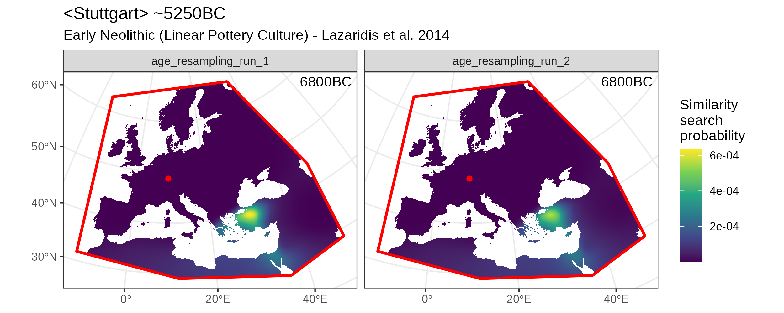
Search results for two different temporal resampling runs.
To finally combine the two age resampling runs we can run fold_probabilities_per_group(), which yields an object of type mobest_locatefold with \(59166/2 = 29583\) rows.
search_sum <- mobest::fold_probabilities_per_group(search_product)
We can plot this final, merged result as usual.
Code for this figure.
ggplot() +
  geom_raster(
    data = search_sum,
    mapping = aes(x = field_x, y = field_y, fill = probability)
  ) +
  scale_fill_viridis_c() +
  geom_sf(
    data = research_area_3035,
    fill = NA, colour = "red",
    linetype = "solid", linewidth = 1
  ) +
  geom_point(
    data = search_samples,
    mapping = aes(x, y),
    colour = "red"
  ) +
  ggtitle(
    label = "<Stuttgart> ~5250BC",
    subtitle = "Early Neolithic (Linear Pottery Culture)\nLazaridis et al. 2014"
  ) +
  theme_bw() +
  theme(
    axis.title = element_blank()
  ) +
  guides(
    fill = guide_colourbar(title = "Similarity\nsearch\nprobability")
  ) +
  annotate(
    "text",
    label = "6800BC",
    x = Inf, y = Inf, hjust = 1.1, vjust = 1.5
  )
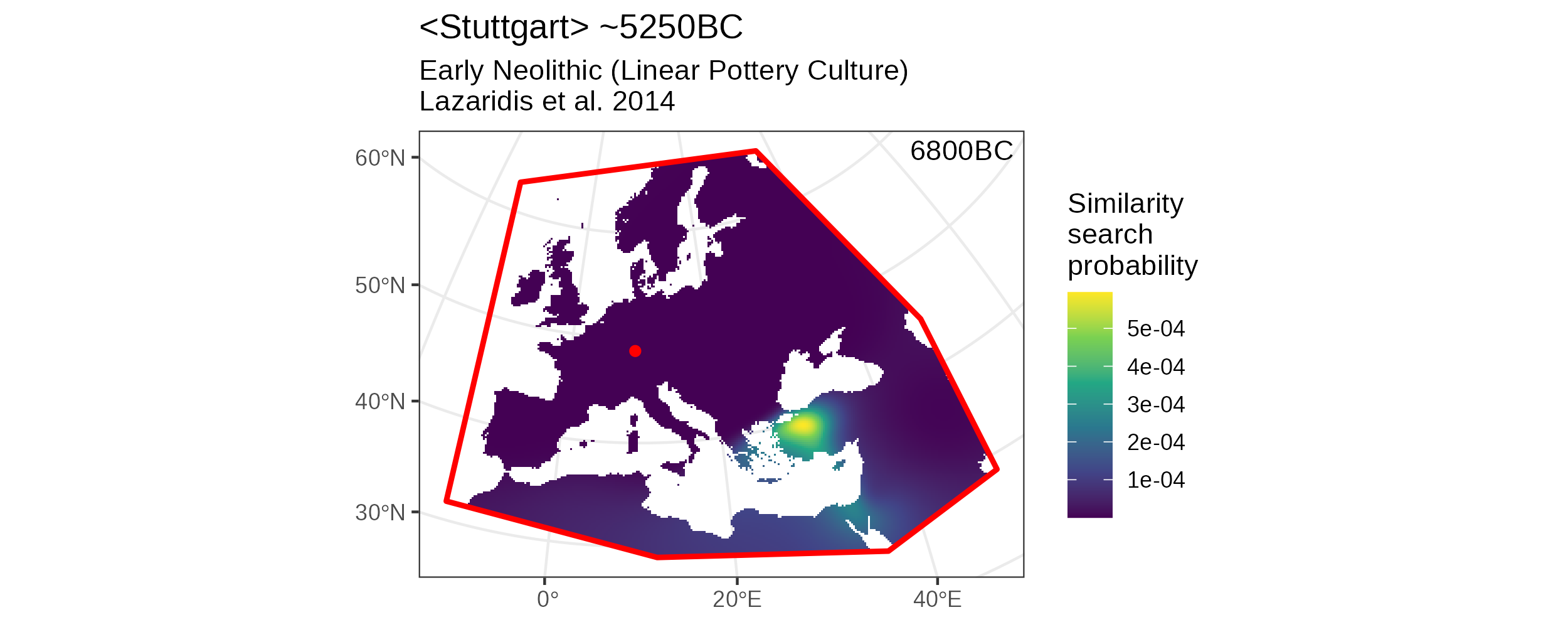
Merged similarity search result based on two temporal resampling runs.