4. Simple permutations

In the example in A basic similarity search workflow we performed the similarity search with mobest::locate() for only one parameter permutation, keeping everything constant except the two dependent variables. But as already laid out above in The mobest_locateoverview table, mobest can automatically consider more parameter permutations, the most basic of which are directly available in locate(). This flexibility has consequences for the presentability of the search results. Here the concept of the origin_vector can be helpful to summarize information.

Warning

Please note that all parameter permutations will be multiplied with all other permutations, causing the number of runs to grow rapidly. If you, for example, submit five time slices and five search samples, the number of runs will be \(5*5=25\) times bigger than for one time slice and sample. The permutation mechanism is explained in more detail in Advanced features of the mobest package.

The following code is included at the end of the similarity_search.R script.

4.1. Multiple search time slices

As explained in Search positions the search_time argument can take an integer vector of relative or absolute ages. That means we can run the search not just for one, but for arbitrarily many time slices with a single call to locate().

Here is an example with two time slices.

search_result <- mobest::locate(
  independent        = ind,
  dependent          = dep,
  kernel             = kernset,
  search_independent = search_ind,
  search_dependent   = search_dep,
  search_space_grid  = spatial_pred_grid,
  search_time        = c(-6800, -5700),
  search_time_mode   = "absolute"
)
search_product <- mobest::multiply_dependent_probabilities(search_result)

Code for this figure.

ggplot() +
  geom_raster(
    data = search_product,
    mapping = aes(x = field_x, y = field_y, fill = probability)
  ) +
  scale_fill_viridis_c() +
  geom_sf(
    data = research_area_3035,
    fill = NA, colour = "red",
    linetype = "solid", linewidth = 1
  ) +
  geom_point(
    data = search_samples,
    mapping = aes(x, y),
    colour = "red"
  ) +
  ggtitle(
    label = "<Stuttgart> ~5250BC",
    subtitle = "Early Neolithic (Linear Pottery Culture) - Lazaridis et al. 2014"
  ) +
  theme_bw() +
  theme(
    axis.title = element_blank()
  ) +
  guides(
    fill = guide_colourbar(title = "Similarity\nsearch\nprobability")
  ) +
  facet_wrap(
    ~search_time,
    labeller = \(variable, value) {
      paste0("Search time: ", abs(value), "BC")
    }
  )

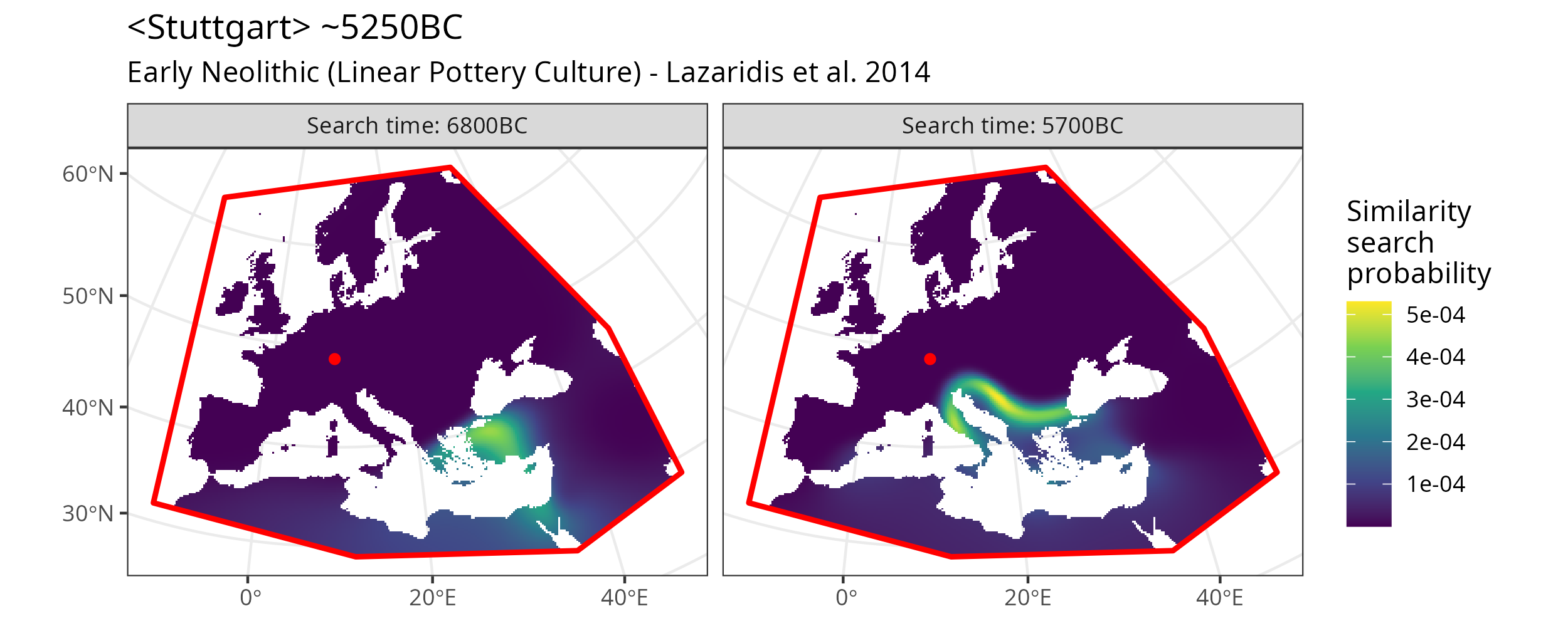
Similarity search map plot for two different time slices.

4.2. Multiple search samples

We can also select multiple search samples and prepare the input data for mobest::locate(). Here we introduce another sample RISE434 originally published in [Allentoft et al., 2015].

search_samples <- samples_projected %>%
  dplyr::filter(
    Sample_ID %in% c("Stuttgart_published.DG", "RISE434.SG")
  )

search_ind <- mobest::create_spatpos(
  id = search_samples$Sample_ID,
  x  = search_samples$x,
  y  = search_samples$y,
  z  = search_samples$Date_BC_AD_Median
)
search_dep <- mobest::create_obs(
  C1 = search_samples$MDS_C1,
  C2 = search_samples$MDS_C2
)

We set the search_time_mode to "relative" to get a different, meaningful search time for both samples.

search_result <- mobest::locate(
  independent        = ind,
  dependent          = dep,
  kernel             = kernset,
  search_independent = search_ind,
  search_dependent   = search_dep,
  search_space_grid  = spatial_pred_grid,
  search_time        = -1500,
  search_time_mode   = "relative"
)
search_product <- mobest::multiply_dependent_probabilities(search_result)

Code for this figure.

ggplot() +
  geom_raster(
    data = search_product,
    mapping = aes(x = field_x, y = field_y, fill = probability)
  ) +
  scale_fill_viridis_c() +
  geom_sf(
    data = research_area_3035,
    fill = NA, colour = "red",
    linetype = "solid", linewidth = 1
  ) +
  geom_point(
    data = search_samples %>% dplyr::rename(search_id = Sample_ID),
    mapping = aes(x, y),
    colour = "red"
  ) +
  theme_bw() +
  theme(
    axis.title = element_blank()
  ) +
  guides(
    fill = guide_colourbar(title = "Similarity\nsearch\nprobability")
  ) +
  facet_wrap(
    ~search_id,
    ncol = 2,
    labeller = labeller(
      search_id = c(
        "Stuttgart_published.DG" = paste(
          "<Stuttgart> ~5250BC",
          "Early Neolithic (Linear Pottery culture) - Lazaridis et al. 2014",
          "Search time: ~6750BC",
          sep = "\n"
        ),
        "RISE434.SG" = paste(
          "<RISE434> ~2750BC",
          "Late Neolithic (Corded Ware culture) - Allentoft et al. 2015",
          "Search time: ~4250BC",
          sep = "\n"
        )
      )
    )
  )

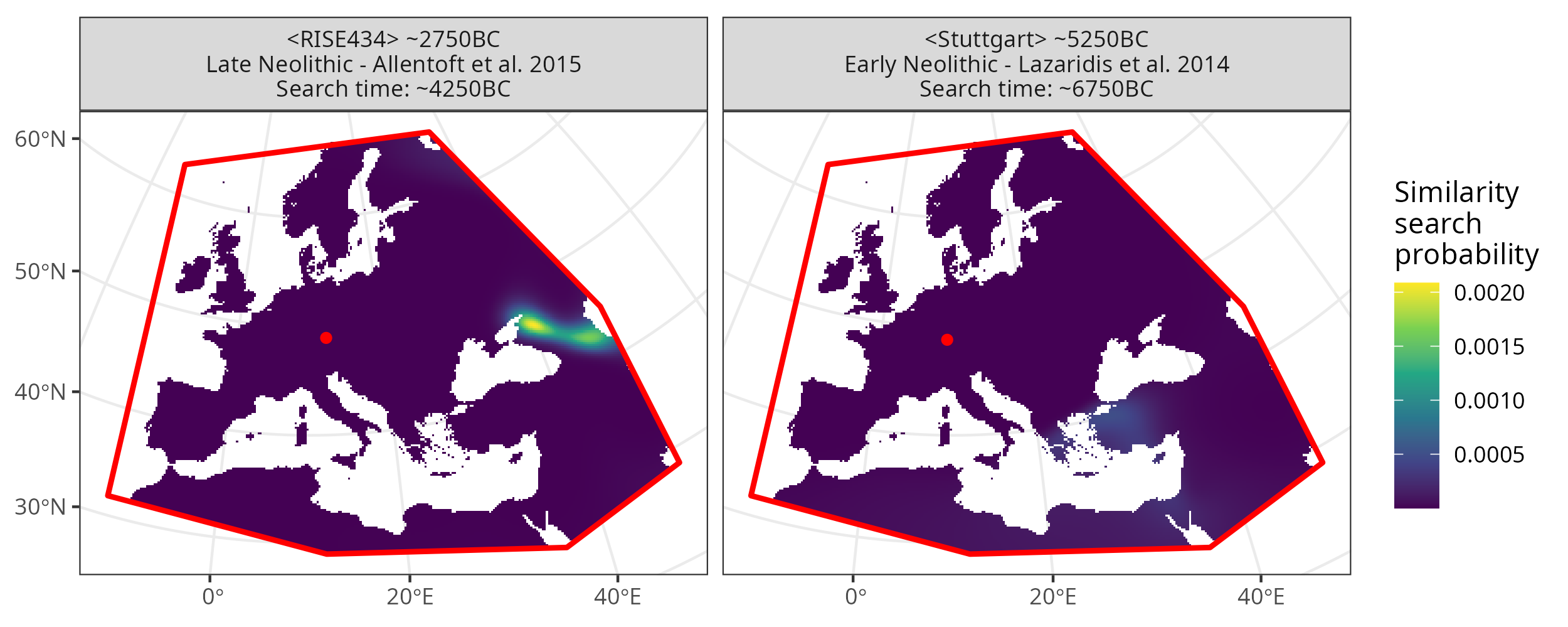
Similarity search map plot for two different search samples.

4.3. Summarizing multiple searches in one figure

Plotting individual similarity probability map plots does not scale well, if the number of searches grows. mobest::determine_origin_vectors() offers a way to derive a simple, summary statistic, by generating what we call origin vectors from objects of class mobest_locateproduct. Each vector connects the spatial point where a sample was found with the point of highest genetic similarity in the interpolated search field and its permutations. The output is of class mobest_originvectors and documents distance and direction of the “origin vector”.

The origin vector summary can also be applied for individual parameter permutations, which is especially relevant for more complex application involving mobest::locate_multi() (see Similarity search with permutations), but already comes in handy for just two different search times, as introduced in the Multiple search time slices section above.

We can take the search_product object from there and apply mobest::determine_origin_vectors() with the grouping variable search_time, to determine one origin vector for each of the two search time iterations.

origin_vectors <- mobest::determine_origin_vectors(search_product, search_time)

The resulting object of type mobest_originvectors features one row for each vector with the following variables.

Column	Description
independent_table_id	Identifier of the spatiotemporal position permutation
dependent_setting_id	Identifier of the dependent variable space position permutation
dependent_var_id	Identifier of the dependent variable
kernel_setting_id	Identifier of the kernel setting permutation
pred_grid_id	Identifier of the spatiotemporal prediction grid
field_id	Identifier of the spatiotemporal prediction point
field_x	Spatial x axis coordinate of the prediction point
field_y	Spatial y axis coordinate of the prediction point
field_z	Temporal coordinate (age) of the prediction point
field_geo_id	Identifier of the spatial prediction point
search_id	Identifier of the search sample
search_x	Spatial x axis coordinate of the search sample
search_y	Spatial y axis coordinate of the search sample
search_z	Temporal coordinate (age) of the search sample
search_time	Search time as provided by the user in locate()’s search_time argument
probability	Probability density calculated in locate()
ov_x	Length of the origin vector in x direction
ov_y	Length of the origin vector in y direction
ov_dist	Length of the origin vector in space (Euclidean distance)
ov_dist_se	Standard error of the mean of all vector lengths
ov_dist_sd	Standard deviation of all vector lengths
ov_angle_deg	Direction of the origin vector as an angle in degree (0-360°)

Warning

Note that here many variables can reflect mean values, as determine_origin_vectors() can summarize information across parameter permutations. Depending on the input mobest_locateproduct table and the specific grouping requirements, multiple origin vectors are determined and then summarized. This explains variables like ov_dist_se and ov_dist_sd, which are only meaningful for groups of vectors.

One basic way of making use of an mobest_originvectors object is by highlighting the points of maximal similarity probability in the map plot.

Code for this figure.

ggplot() +
  geom_raster(
    data = search_product,
    mapping = aes(x = field_x, y = field_y, fill = probability)
  ) +
  scale_fill_viridis_c() +
  geom_sf(
    data = research_area_3035,
    fill = NA, colour = "red",
    linetype = "solid", linewidth = 1
  ) +
  geom_point(
    data = search_samples,
    mapping = aes(x, y),
    colour = "red"
  ) +
  geom_point(
    data = origin_vectors,
    mapping = aes(field_x, field_y),
    fill = "orange", shape = 24
  ) +
  geom_segment(
    data = origin_vectors,
    mapping = aes(
      x = search_x, y = search_y,
      xend = field_x, yend = field_y
    ),
    arrow = arrow(length = unit(0.2, "cm")),
    colour = "red"
  ) +
  geom_label(
    data = origin_vectors,
    mapping = aes(
      x = (field_x + search_x)/2, y = (field_y + search_y)/2,
      label = paste0(round(ov_dist/1000, -2), "km")
    ),
    fill = "white", colour = "red", size = 2
  ) +
  ggtitle(
    label = "<Stuttgart> ~5250BC",
    subtitle = "Early Neolithic (Linear Pottery Culture) - Lazaridis et al. 2014"
  ) +
  theme_bw() +
  theme(
    axis.title = element_blank()
  ) +
  guides(
    fill = guide_colourbar(title = "Similarity\nsearch\nprobability")
  ) +
  facet_wrap(
    ~search_time,
    labeller = \(variable, value) {
      paste0("Search time: ", abs(value), "BC")
    }
  )

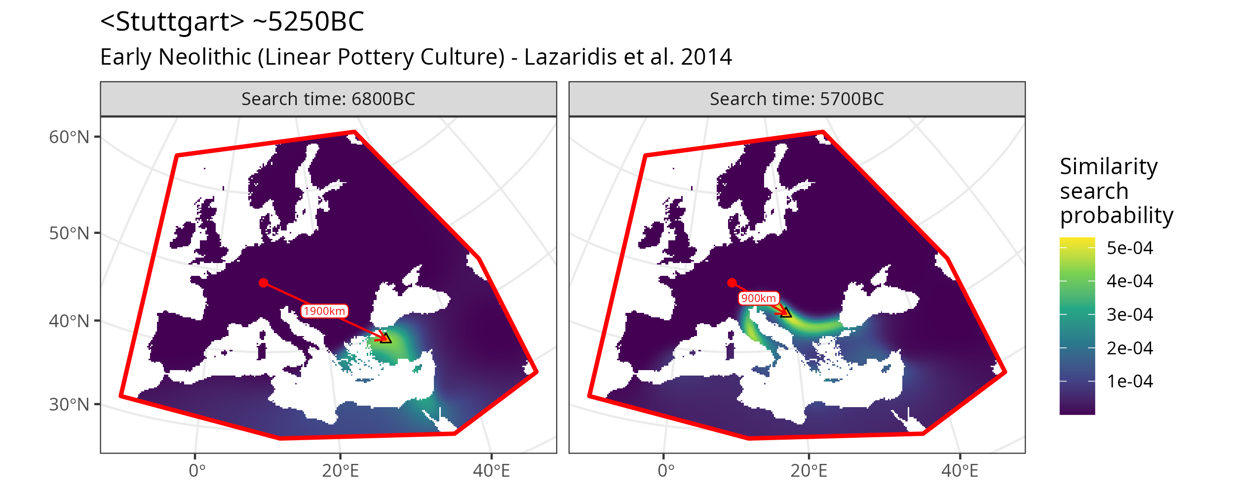
Similarity search map plot for two different time slices including arrows to the point of maximum similarity probability. cf. Figure ‘Similarity search map plot for two different time slices.’

With origin_vectors we can also summarize the results for two different samples, as in Multiple search samples above, in a single figure.

If we take the search_product object from there and apply mobest::determine_origin_vectors() without a grouping variable - grouping by sample is the default - then we get origin vectors for the two samples, which we can display in the same map figure.

origin_vectors <- mobest::determine_origin_vectors(search_product)

Code for this figure.

ggplot() +
  geom_sf(
    data = research_land_outline_3035,
    fill = "grey", color = NA
  ) +
  geom_sf(
    data = research_area_3035,
    fill = NA, colour = "red",
    linetype = "solid", linewidth = 1
  ) +
  geom_point(
    data = origin_vectors,
    mapping = aes(search_x, search_y),
    colour = "red"
  ) +
  geom_point(
    data = origin_vectors,
    mapping = aes(field_x, field_y),
    fill = "orange", shape = 24
  ) +
  geom_segment(
    data = origin_vectors,
    mapping = aes(
      x = search_x, y = search_y,
      xend = field_x, yend = field_y
    ),
    arrow = arrow(length = unit(0.2, "cm")),
    colour = "red"
  ) +
  theme_bw() +
  theme(
    axis.title = element_blank()
  )

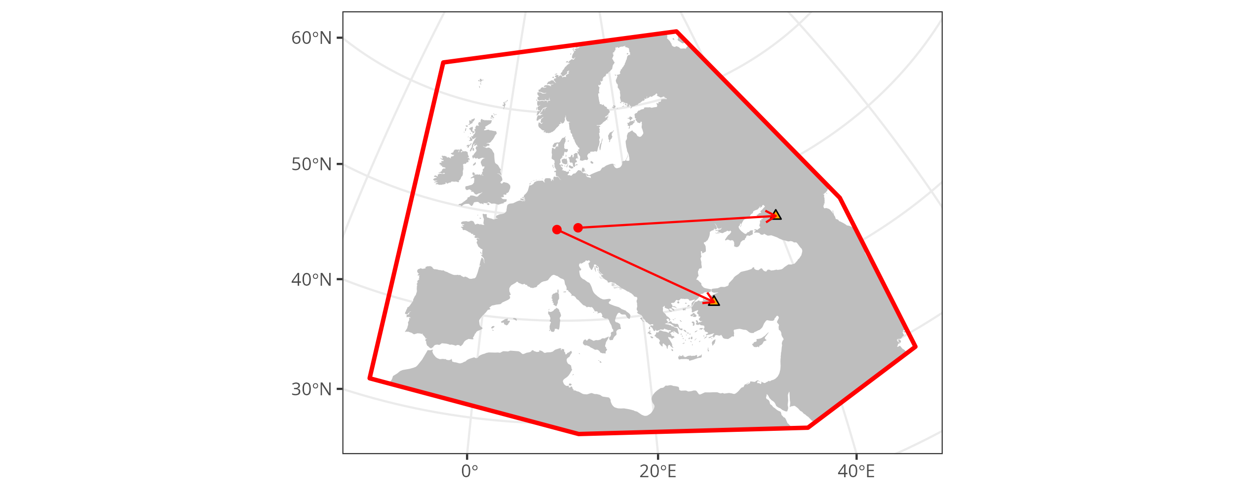
Prototype of a figure that combines the independent search results for two samples in one figure. cf. Figure ‘Similarity search map plot for two different search samples.’