5. Parameter estimation for optimal ancestry interpolation

One important question for the Gaussian process regression performed within multiple of the core functions of mobest is how to find correct and useful settings for the kernel hyperparameters (see Kernel parameter settings in the basic workflow description). Supplementary Text 2 of [Schmid and Schiffels, 2023] discusses this in detail. Based on this mobest provides different helper functions to either estimate the parameters or prepare data products that can be used to estimate them. Here we explain a practical way to estimate the nugget and lengthscale values.

For this tutorial we will use the data introduced and prepared in A basic similarity search workflow, specifically a samples_projected.csv table prepared in Reading the input samples.

You can download the script with the main workflow explained below including the required test data:

• parameter_estimation.R

• samples_projected.csv

5.1. Preparing the computational environment

We start by loading the required packages we do not want to call explicitly from their source namespaces.

library(magrittr)
library(ggplot2)

For more information see the Preparing the computational environment section in the basic tutorial.

5.2. Using a subset of the variogram to estimate the nugget parameter

We then load the input data: individual ancient DNA samples with their spatiotemporal and genetic position.

samples_projected <- readr::read_csv("docs/data/samples_projected.csv")
# you have to replace "data/docs/" with the path to your copy of the file

5.2.1. Determining pairwise distances

mobest::calculate_pairwise_distances() allows to calculate different types of pairwise distances (spatial, temporal, dependent variables/ancestry components) for each input sample pair and returns them in a long format tibble of class mobest_pairwisedistances.

distances_all <- mobest::calculate_pairwise_distances(
  independent = mobest::create_spatpos(
    id = samples_projected$Sample_ID,
    x = samples_projected$x,
    y = samples_projected$y,
    z = samples_projected$Date_BC_AD_Median
  ),
  dependent = mobest::create_obs(
    C1 = samples_projected$MDS_C1,
    C2 = samples_projected$MDS_C2
  )
)

Helper functions are available to calculate the individual types of distances, if this is desired.

geo_dist  <- mobest::calculate_geo_pairwise_distances(positions)
time_dist <- mobest::calculate_time_pairwise_distances(positions)
obs_dist  <- mobest::calculate_dependent_pairwise_distances(positions$id, observations)

Warning

Spatial distances (from calculate_geo_pairwise_distances()) are assumed to be in meter and transformed to kilometres. As this can be inaccurate (see Projecting the spatial data) the feature can be turned off with m_to_km = FALSE.

Warning

mobest::calculate_pairwise_distances() calculates the distances in dependent variables space on the residuals of a linear model informed from the spatiotemporal positions and returns it in a set of columns with the suffix *_dist_resid (see Gaussian process regression on top of a linear model). This behaviour can be turned off by setting with_resid = FALSE.

mobest_pairwisedistances, here in distances_all, includes the following columns/variables.

Column	Description
id1	Identifier of the first sample
id2	Identifier of the second sample
geo_dist	Spatial distance (in the units of the CRS, typically kilometres)
time_dist	Temporal distance (typically in years)
obs_dist_total	Euclidean distance in the dependent variable space, so across all dimensions
*_dist	Distance along the axis of one dependent variable denoted by *
*_dist_resid	Distance along the axis of one dependent variable, but here only the distance in the space defined by the residuals of a linear model

The mobest_pairwisedistances table allows us to easily visualize and analyse the pairwise distance properties of our dataset, for example with scatter plots or 2D histograms.

Code for this figure.

p1 <- ggplot() +
  geom_bin2d(
    data = distances_all,
    mapping = aes(x = geo_dist, y = obs_dist_total),
    bins = 30
  ) +
  scale_fill_viridis_c() +
  theme_bw()

p2 <- ggplot() +
  geom_bin2d(
    data = distances_all,
    mapping = aes(x = time_dist, y = obs_dist_total),
    bins = 30
  ) +
  scale_fill_viridis_c() +
  theme_bw()

cowplot::plot_grid(p1, p2)

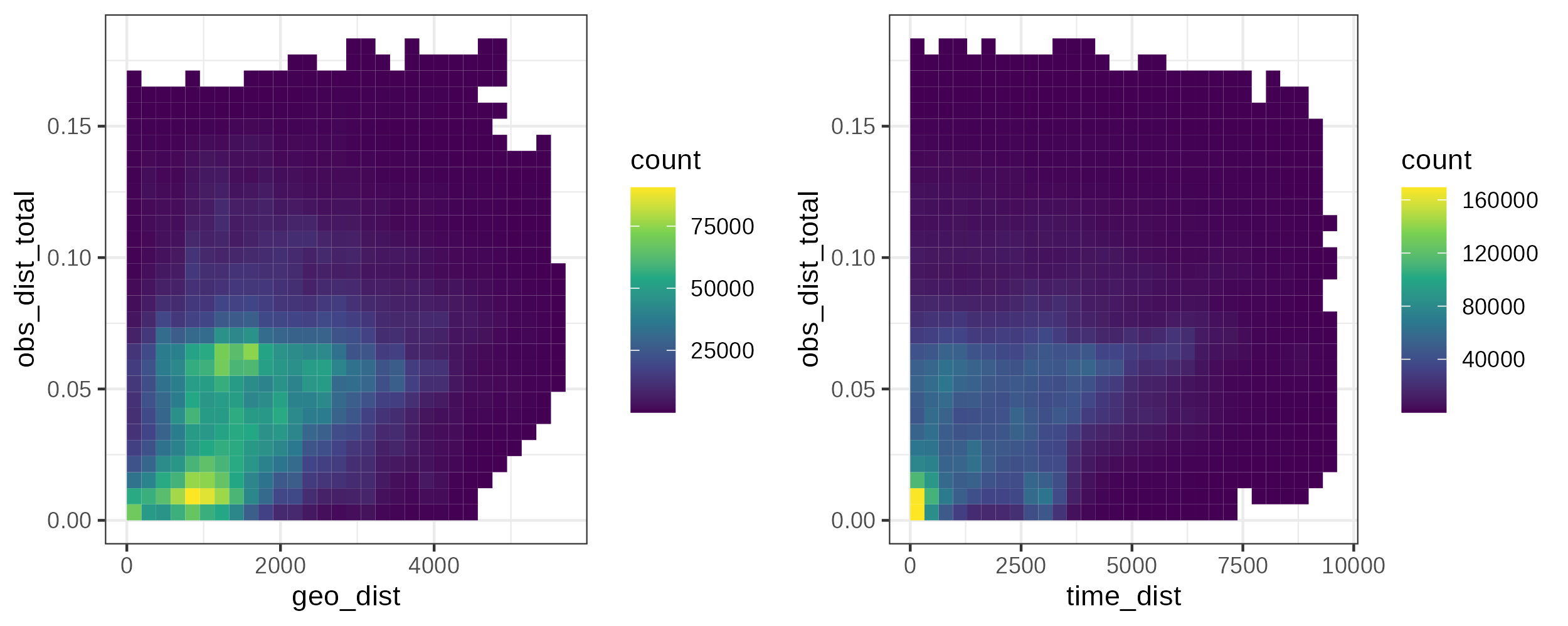
2D histograms of the sample distance pairs comparing spatial (geo_dist), temporal (time_dist) and genetic (obs_dist) space.

5.2.2. Summarizing distances in an empirical variogram

mobest::bin_pairwise_distances() bins the pairwise distances in a mobest_pairwisedistances object according to spatial and temporal distance categories and calculates an empirical variogram of class mobest_empiricalvariogram for the Euclidean distances in the genetic dependent variable space. geo_bin and time_bin set the spatial and temporal bin size. The per_bin_operation to summarize the information is per-default set to function(x) { 0.5 * mean(x^2, na.rm = T) }, so half the mean squared value of all genetic distances in a given bin.

variogram <- mobest::bin_pairwise_distances(
  distances_all,
  geo_bin = 100, time_bin = 100
)

mobest_empiricalvariogram includes these columns/variables.

Column	Description
geo_dist_cut	Upper bound of the spatial bin
time_dist_cut	Upper bound of the temporal bin
obs_dist_total	Euclidean distance in the dependent variable space, summarized with the per_bin_operation
C*_dist	Distance in along the axis of one dependent variable, summarized with the per_bin_operation
C*_dist_resid	Distance in residual space for one dependent variable, summarized with the per_bin_operation
n	Number of pairwise distances in a given space-time bin (as already shown in 2D histograms of the sample distance pairs comparing spatial (geo_dist), temporal (time_dist) and genetic (obs_dist) space.)

5.2.3. Estimating the nugget parameter

One form of the variogram can be used to estimate the nugget parameter of the GPR kernel settings, by filtering for pairwise “genetic” distances with very small spatial and temporal distances. Here is one workflow to do so.

distances_for_nugget <- distances_all %>%
  # remove self-distances
  dplyr::filter(id1 != id2) %>%
  # filter for small temporal and spatial pairwise distances
  dplyr::filter(time_dist < 50 & geo_dist < 50) %>%
  # transform the residual dependent variable distances
  # into a long format table
  tidyr::pivot_longer(
    cols = tidyselect::ends_with("_resid"),
    names_to = "dist_type", values_to = "dist_val"
  ) %>%
  # rescale the distances to relative proportions
  dplyr::mutate(
    dist_val_adjusted = dplyr::case_when(
      dist_type == "C1_dist_resid" ~
        0.5*(dist_val^2 / stats::var(samples_projected$MDS_C1)),
      dist_type == "C2_dist_resid" ~
        0.5*(dist_val^2 / stats::var(samples_projected$MDS_C2))
    )
  )

We remove the zero-distances from samples to themselves and then filter to very small spatial and temporal distances, so to pairs of samples that are very close in space and time. Within this subset we rescale the distances in dependent variable space, so genetic distances, to reflect a proportion of the variance of the samples in said space.

The mean of the resulting metric can be employed as the nugget value for a given dependent variable.

estimated_nuggets <- distances_for_nugget %>%
  dplyr::group_by(dist_type) %>%
  dplyr::summarise(nugget = mean(dist_val_adjusted, na.rm = T))

# estimated_nuggets
# A tibble: 2 × 2
  dist_type     nugget
  <chr>          <dbl>
1 C1_dist_resid 0.0710
2 C2_dist_resid 0.0589

Code for this figure.

ggplot() +
  geom_violin(
    data = distances_for_nugget,
    mapping = aes(x = dist_type, y = dist_val_adjusted, fill = dist_type),
    linewidth = 0.5,
    width = 0.8
  ) +
  geom_boxplot(
    data = distances_for_nugget,
    mapping = aes(x = dist_type, y = dist_val_adjusted),
    width = 0.1, outlier.size = 1
  ) +
  geom_point(
    data = estimated_nuggets,
    mapping = aes(x = dist_type, y = nugget),
    size = 4, shape = 18
  ) +
  geom_point(
    data = estimated_nuggets,
    mapping = aes(x = dist_type, y = nugget),
    size = 6, shape = "|"
  ) +
  geom_text(
    data = estimated_nuggets,
    mapping = aes(x = dist_type, y = nugget, label = paste0("mean: ~", round(nugget, 3))),
    nudge_x = -0.5
  ) +
  coord_flip() +
  theme_bw() +
  guides(fill = "none") +
  xlab("ancestry component distance type") +
  ylab("pairwise half mean squared normalized residual distance") +
  scale_y_log10(labels = scales::comma) +
  scale_x_discrete(limits = rev(unique(distances_for_nugget$dist_type)))

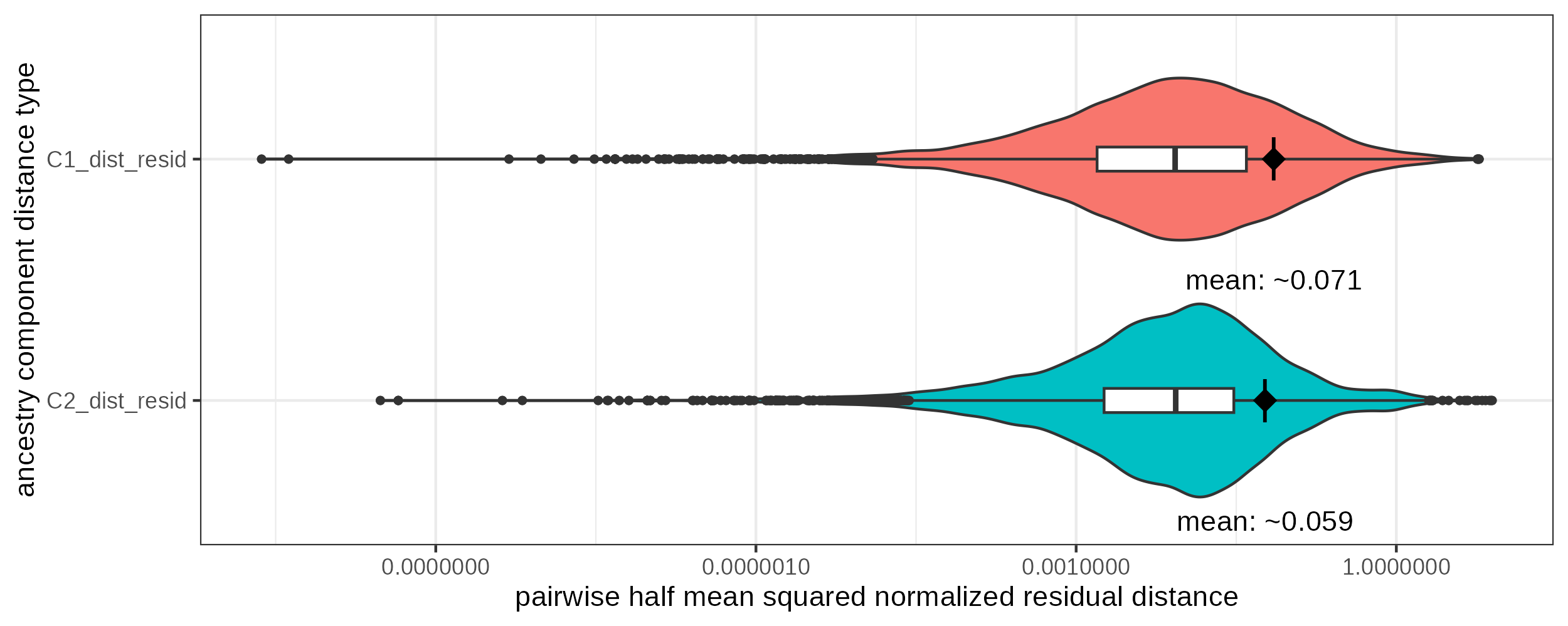
Violin- and boxplot of the detrended pairwise distance distribution for different ancestry components in a short and narrow temporal and spatial distance window (< 50km & < 50years). The diamond shaped dot is positioned at the mean point of the distribution

5.3. Finding optimal lengthscale parameters with crossvalidation

To find the empirically optimal lengthscale parameters mobest includes the function mobest::crossvalidate(). It allows to tackle the parameter estimation challenge with simple crossvalidation across a grid of kernel parameters. This is a computationally expensive and mathematically inelegant method, but robust, reliable and readily understandable. crossvalidate() internally employs mobest::create_model_grid() and mobest::run_model_grid() (see Spatiotemporal interpolation permutations in a model grid).

For the following example code we can speed up the expensive calculations by reducing the sample size.

set.seed(123)
samples_reduced <- samples_projected %>% dplyr::slice_sample(n = 100)
# typically one would run this with all available samples

5.3.1. A basic crossvalidation setup

To run mobest::crossvalidate() we require the spatiotemporal and dependent, genetic variable coordinates of the field-informing input samples, fixed nuggets for each dependent variable and a grid of kernel parameters to explore.

The input positions can be specified as objects of type mobest_spatiotemporalpositions and mobest_observations just as laid out for mobest::locate() (see Independent and dependent positions).

ind <- mobest::create_spatpos(
  id = samples_reduced$Sample_ID,
  x  = samples_reduced$x,
  y  = samples_reduced$y,
  z  = samples_reduced$Date_BC_AD_Median
)
dep <- mobest::create_obs(
  C1 = samples_reduced$MDS_C1,
  C2 = samples_reduced$MDS_C2
)

The grid of kernel parameters grid is a bit more difficult to obtain. It has to be of type mobest_kernelsetting_multi (see Permutation data types), which is a bit awkward to construct for a large set of value permutations. Here is one way of doing so:

kernels_to_test <-
  # create a permutation grid of spatial (ds) and temporal (dt) lengthscale parameters
  expand.grid(
    ds = seq(100, 1900, 200)*1000, # *1000 to transform from kilometres to meters
    dt = seq(100, 1900, 200)
  ) %>%
  # create objects of type mobest_kernelsetting from them
  purrr::pmap(function(...) {
    row <- list(...)
    mobest::create_kernset(
      C1 = mobest::create_kernel(
        dsx = row$ds,
        dsy = row$ds,
        dt  = row$dt,
        g   = 0.071  # nugget for C1 as calculated above 
      ),
      C2 = mobest::create_kernel(
        dsx = row$ds,
        dsy = row$ds,
        dt  = row$dt,
        g   = 0.059
      )
    )
  }) %>%
  # name then and  package them in an object of type mobest_kernelsetting_multi
  magrittr::set_names(paste("kernel", 1:length(.), sep = "_")) %>%
  do.call(mobest::create_kernset_multi, .)

Note

The kernel grid explored here is coarse-meshed: kernels_to_test includes \(10 * 10 = 100\) different kernel settings. Finer grids are advisable for real-world applications. To reduce the computational workload a multi-step approach can be useful: First investigating a very large but coarse lengthscale parameter grid, and then submitting a second or even a third run with a “zoomed-in” grid in the area with the best interpolation model performance.

With this input ready we can call mobest::crossvalidate(). This function randomly splits the input data in a number of groups as defined by the groups argument, takes groups - 1 of them as training data and uses it to estimate the dependent variable positions of the last group’s samples. It then calculates the differences between the true and the predicted values for each test sample and documents it in a tabular data structure of type mobest_interpolgrid. This is repeated so that each group acts as the test group once, so each sample is predicted by the others once. In another iteration this entire process is repeated after resampling the groups.

Warning

Even this extremely reduced example may run for several minutes, depending on your system.

interpol_comparison <- mobest::crossvalidate(
  independent = ind,
  dependent   = dep,
  kernel      = kernels_to_test,
  iterations  = 2, # in a real-world setting this should be set to 10+ iterations
  groups      = 5, # and this to 10
  quiet       = F
)

That means each row in interpol_comparison features the result for one test sample with one kernel parameter permutation and iteration. The following variables are documented:

Column	Description
independent_table_id	Identifier of the spatiotemporal position permutation
dependent_setting_id	Identifier of the dependent variable space position permutation
dependent_var_id	Identifier of the dependent variable
kernel_setting_id	Identifier of the kernel setting permutation
pred_grid_id	Identifier of the spatiotemporal prediction grid
mixing_iteration	Number of iteration
dsx	Kernel lengthscale parameter on the spatial x axis
dsy	Kernel lengthscale parameter on the spatial y axis
dt	Kernel lengthscale parameter on the temporal axis
g	Kernel nugget parameter
id	Identifier of the test sample
x	Spatial x axis coordinate of the test sample
y	Spatial y axis coordinate of the test sample
z	Temporal coordinate (age) of the test sample
mean	Mean value predicted by the GPR model for the dependent variable at the location of the test sample
sd	Uncertainty predicted by the GPR model for the dependent variable at the location of the test sample
measured	Genetic coordinate of the test sample in the dependent variable space
difference	Difference between mean (the predicted value) and measured (the actually observed value)

interpol_comparison has \(2 * 100 * 100 * 2 = 40000\) rows as a result of the following permutations:

• \(2\) dependent variables

• \(100\) set of kernel parameter settings

• \(100\) spatial prediction grid positions

• \(2\) group resampling iterations

5.3.2. Analysing the crossvalidation results

To finally decide which kernel parameters yield the overall best prediction we have to summarize the per-sample results in the mobest_interpolgrid table. One way of doing this is by calculating the mean-squared difference for each lenghtscale setting.

kernel_grid <- interpol_comparison %>%
  dplyr::group_by(
    dependent_var_id, ds = dsx, dt) %>%
  dplyr::summarise(
    mean_squared_difference = mean(difference^2),
    .groups = "drop"
  )

And this can then be visualized in a raster plot.

Code for this figure.

p1 <- ggplot() +
  geom_raster(
    data = kernel_grid %>% dplyr::filter(dependent_var_id == "C1"),
    mapping = aes(x = ds / 1000, y = dt, fill = mean_squared_difference)
  ) +
  scale_fill_viridis_c(direction = -1) +
  coord_fixed() +
  theme_bw() +
  xlab("spatial lengthscale parameter") +
  ylab("temporal lengthscale parameter") +
  guides(
    fill = guide_colourbar(title = "Mean squared\ndifference\nbetween\nprediction &\ntrue value")
  ) +
  ggtitle("C1")

p2 <- ggplot() +
  geom_raster(
    data = kernel_grid %>% dplyr::filter(dependent_var_id == "C2"),
    mapping = aes(x = ds / 1000, y = dt, fill = mean_squared_difference)
  ) +
  scale_fill_viridis_c(direction = -1) +
  coord_fixed() +
  theme_bw() +
  xlab("spatial lengthscale parameter") +
  ylab("temporal lengthscale parameter") +
  guides(
    fill = guide_colourbar(title = "Mean squared\ndifference\nbetween\nprediction &\ntrue value")
  ) +
  ggtitle("C2")

cowplot::plot_grid(p1, p2)

Crossvalidation results (mean squared differences between prediction and observation) for two dependent variables/ancestry components C1 and C2

The very best parameter combination for each dependent variable can be identified like this:

kernel_grid %>%
  dplyr::group_by(dependent_var_id) %>%
  dplyr::slice_min(order_by = mean_squared_difference, n = 1) %>%
  dplyr::ungroup()

# A tibble: 2 × 4
  dependent_var_id      ds    dt mean_squared_difference
  <chr>              <dbl> <dbl>                   <dbl>
1 C1               1100000  1500                0.000320
2 C2               1900000  1900                0.000131

Note that these values here are just for demonstration and a result of a crossvalidation run with a very small sample size. Extremely large kernel sizes are plausible for extremely small sample density.

5.4. An HPC crossvalidation setup for large lengthscale parameter spaces

The setup explained above is complete, but impractical for applications with large datasets and a large relevant parameter space. If you have access to a desktop computer or a single, strong node on a HPC system with plenty of processor cores, then it might be feasible to call the R code introduced above there. This hardly scales to really large analyses, though. For that we require a distributed computing setup, which makes use of the multitude of individual nodes a typical HPC provides.

Here is an example for a HPC setup where the workload for a large crossvalidation analysis is distributed across many individual jobs. This setup has three components, which will be explained in detail below.

1. An R script specifying the individual crossvalidation run: cross.R

2. A bash script to call 1. through the scheduler with a sequence of parameters: run.sh

3. An R script to compile the output of the many calls to 1. into a table like the kernel_grid object above: compile.R

Warning

To make sure this example actually works, we filled it with real paths. Make sure to change them for your application.

5.4.1. The crossvalidation R script

The following script cross.R includes the code for a single run of the crossvalidation with one set of kernel parameters.

Note how the command line arguments are read from run.sh with base::commandArgs() and then used in mobest::create_kernset() to run mobest::crossvalidate() with exactly the desired lengthscale parameters.

# load dependencies
library(magrittr)

# read command line parameters
args <- unlist(strsplit(commandArgs(trailingOnly = TRUE), " "))
run <- args[1]
ds_for_this_run <- as.numeric(args[2])
dt_for_this_run <- as.numeric(args[3])

# read samples
samples_projected <- readr::read_csv(
  "docs/data/samples_projected.csv"
)

# transform samples to the required input data types
ind <- mobest::create_spatpos(
  id = samples_projected$Sample_ID,
  x  = samples_projected$x,
  y  = samples_projected$y,
  z  = samples_projected$Date_BC_AD_Median
)
dep <- mobest::create_obs(
  C1 = samples_projected$MDS_C1,
  C2 = samples_projected$MDS_C2
)

# define the kernel for this run
kernel_for_this_run <- mobest::create_kernset_multi(
  mobest::create_kernset(
    C1 = mobest::create_kernel(
      dsx = ds_for_this_run*1000,
      dsy = ds_for_this_run*1000,
      dt  = dt_for_this_run,
      g   = 0.071
    ),
    C2 = mobest::create_kernel(
      dsx = ds_for_this_run*1000,
      dsy = ds_for_this_run*1000,
      dt  = dt_for_this_run,
      g   = 0.059
    )
  ),
  .names = paste0("kernel_", run)
)

# set a seed to freeze randomness
set.seed(123)
# the only random element of this analysis is the splitting into sample groups 
# with this seed the groups should be identical for each parameter configuration

# run crossvalidation
interpol_comparison <- mobest::crossvalidate(
  independent = ind,
  dependent   = dep,
  kernel      = kernel_for_this_run,
  iterations  = 10,
  groups      = 10,
  quiet       = F
)

# summarize the crossvalidation result
kernel_grid <- interpol_comparison %>%
  dplyr::group_by(
    dependent_var_id, ds = dsx, dt) %>%
  dplyr::summarise(
    mean_squared_difference = mean(difference^2),
    .groups = "drop"
  )

# write the output to the file system
readr::write_csv(
  kernel_grid,
  file = paste0(
    "docs/data/hpc_crossvalidation/kernel_grid_",
    sprintf("%06d", as.integer(run)),
    ".csv"
  )
)

cross.R returns a very short table (in the script the object kernel_grid of type mobest_interpolgrid) with only two lines; one for each dependent variable. It writes it to the file system as a .csv file with a unique name: kernel_grid_000XXX.csv, where XXX is the run number.

For testing purposes is possible to run this script with a specific set of lengthscale parameters, here 1000 kilometres and 1000 years.

Rscript /mnt/archgen/users/schmid/mobest/docs/data/hpc_crossvalidation/cross.R "999" "1000" "1000"

If the local R installation does not already include the mobest package, we may want to run Rscript through apptainer, as described in Create an apptainer image to run mobest.

apptainer exec \
  --bind=/mnt/archgen/users/schmid/mobest \
  /mnt/archgen/users/schmid/mobest/apptainer_mobest.sif \
  Rscript /mnt/archgen/users/schmid/mobest/docs/data/hpc_crossvalidation/cross.R "999" "1000" "1000" \
  /

And if we want to go all the way, we can also submit this to the HPC scheduler, in this case SGE.

qsub -b y -cwd -q archgen.q -pe smp 10 -l h_vmem=20G -now n -V -j y -o ~/log -N crossOne \ 
  apptainer exec \
    --bind=/mnt/archgen/users/schmid/mobest \
    /mnt/archgen/users/schmid/mobest/apptainer_mobest.sif \
    Rscript /mnt/archgen/users/schmid/mobest/docs/data/hpc_crossvalidation/cross.R "999" "1000" "1000" \
    /

5.4.2. The submission bash script

Of course we usually do not want to run cross.R only once, but many times for a regular grid of lengthscale parameters. The following SGE submission script run.sh now describes how the R script can be submitted to a scheduler as an array of jobs. It can be submitted with qsub docs/data/hpc_crossvalidation/run.sh.

Note how the parameter grid is constructed by two nested loops and indexed by the SGE_TASK_ID, more specifically SGE_TASK_ID - 1 = i. The number of jobs, here \(15*15=225\), is hardcoded in -t 1-225 and must be calculated and set in advance based on the number of values in ds_to_explore and dt_to_explore. seq 100 100 1500 creates a sequence of 15 values from 100 to 1500 in steps of 100.

#!/bin/bash
#
#$ -S /bin/bash  # defines bash as the shell for execution
#$ -N cross      # name of the command that will be listed in the queue
#$ -cwd          # change to the current directory
#$ -j y          # join error and standard output in one file
#$ -o ~/log      # standard output file or directory
#$ -q archgen.q  # queue
#$ -pe smp 2     # use X CPU cores
#$ -l h_vmem=10G # request XGb of memory
#$ -V            # load personal profile
#$ -t 1-225      # array job length
#$ -tc 25        # number of concurrently submitted tasks

date

echo Task in Array: ${SGE_TASK_ID}
i=$((SGE_TASK_ID - 1))

# determine parameter permutations
ds_to_explore=($(seq 100 100 1500))
dt_to_explore=($(seq 100 100 1500))
dss=()
dts=()
for ds in "${ds_to_explore[@]}"
do
  for dt in "${dt_to_explore[@]}"
  do
    dss+=($ds)
    dts+=($dt)
  done
done
current_ds=${dss[${i}]}
current_dt=${dts[${i}]}

echo ds: ${current_ds}
echo dt: ${current_dt}

apptainer exec \
  --bind=/mnt/archgen/users/schmid/mobest \
  /mnt/archgen/users/schmid/mobest/apptainer_mobest.sif \
  Rscript /mnt/archgen/users/schmid/mobest/docs/data/hpc_crossvalidation/cross.R ${i} ${current_ds} ${current_dt} \
  /

date
exit 0

So this will start 225 jobs in batches of 25 jobs at a time. Each job will run cross.R with a different set of input parameters, which will, in turn, create 225 kernel_grid_000XXX.csv files.

5.4.3. The result compilation script

To read these individual files, and subsequently create the plot described in Analysing the crossvalidation results a third script compile.R is in order. It should probably start with some code like this, which reads and merges the individual files into a single data structure.

kernel_grid <- purrr::map_dfr(
  list.files(
    path = "docs/data/hpc_crossvalidation",
    pattern = "*.csv",
    full.names = TRUE
  ),
  function(x) {
    readr::read_csv(x, show_col_types = FALSE)
  }
)